Conformal predictions
Intro
This article is a small summary of my notes regarding conformal predictions. Conformal predictions is the new kid on the block in the “measuring uncertainty field” in machine learning.
Conformal prediction is a framework in machine learning and statistical inference that provides a way to quantify and control the confidence or reliability of predictions made by a model. It aims to address the limitations of traditional point predictions, which only provide a single prediction without any measure of uncertainty.
Motivation
Usually we expect past performance to be a good indicator for future performance. We build a training set, and evaluate our algorithm on a test set and we hope that this represents the context of future predictions.
We estimate how it will work on future data by testing it on data that we know today, so basically we expect past performance to estimate future performance.
For instance… The model has a AUC score of 0.9 on the test set and we expect an AUC score of 0.9 on unseen future data.
But how good are these estimates? Do we have any guarantees? We have a score that is actually telling us something on average (for instance a 90% accuracy on the test test). We really care about how good a prediction is on a single new point and how confident can we be about this new prediction?
A practical example regarding uncertainty
Let’s take a simple example where you have a neural network that examines an MRI to detect a tumor in the brain. Let’s say our neural network is learned to classify an image into 3 categories / labels :
- Normal
- Tumor detected
- Concussion
A neural network can have a cross-entropy loss function that will give back a number between 0 and 1 and this number will represents a concept of confidence. For highly critical decision making this is a problem since we have no assurance that our model is well-calibrated in terms of their predicted probabilities. This means that a score 0.8 does not necessarily correspond to an 80% confidence level in the true label.
There are several ways to address this problem like bayesian networks, model calibration, etc but in this article we will look at conformal predictions.
Conformal predictions don’t give you a confidence number for a single prediction, but give you a set of predictions for which we are X percent certain that the true label is in that set.
For our case let’s examine both and see which is more useful for a doctor.
Traditional prediction:
- Normal 0.9
- Tumor detected 0.05
- Concussion 0.05
Conformal prediction:
We are ≥ 90% sure that this patient has one of the options of this set:
[ Normal, Tumor, Concussion ]
In the below case you will be more tempted to accept that you are not certain enough to assume that there is no tumor and further analysis is required.
What is so special about conformal predictions?
The big difference with other approaches is that you don’t need to analyse your model and don’t need to (re)train the model multiple times (model calibration, ensemble methods, etc) and the model itself doesn’t need to have robust uncertainty incorporated (bayesian networks). The model is a black box in this approach.
Concepts in the context of classification
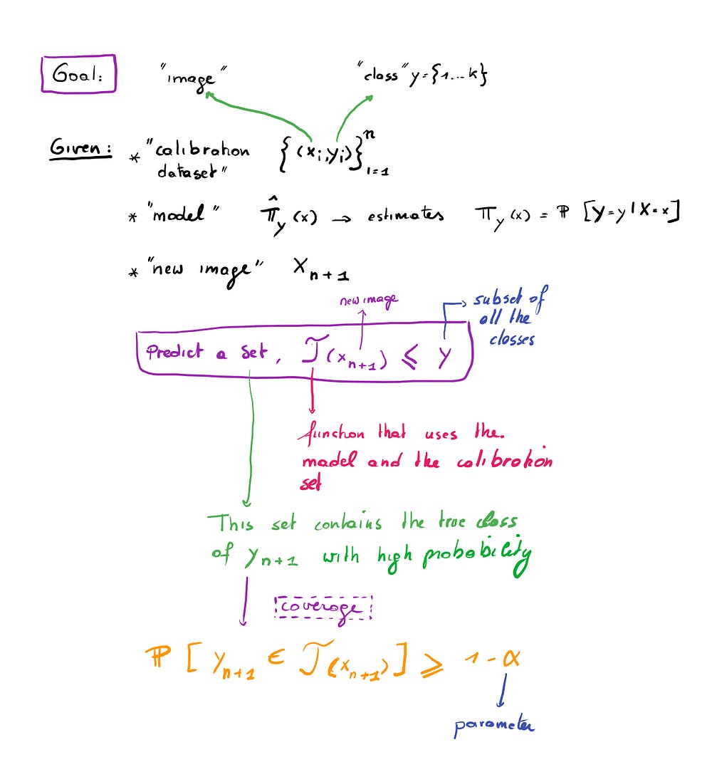
We have a classification of images and for conformal predictions we need the following:
- A calibration set of size n (where n is a finite small portion of the data set). This calibration set is never seen by the model.
- A model which estimates the probability distribution for each potential classification label (we have k labels in the example below).
- A new image Xₙ₊₁ that we will use for a conformal prediction

We now have a function T that takes in a new image and predicts a set which contains a subset of all the possible classes.
This function T uses the model and the calibration set and the predicted set contains the true class for the new image with high probability.
The probability can be controlled by x which is a parameter, so if we take x to be 0.1, then we have 90% probability that our image has a classification class which is present in the set that is given by the function T.
Let’s see an example:

Image 1: We are sure that it’s a squirrel and the prediction set also contains only one image
Image 2: We are less sure than in image 1 and our prediction set grows to 4 classes
Image 3: We are not certain at all and our prediction set contains 6 classes.
Basic simple algorithm
Let’s see how we can construct that function T that appears to do all the magic.
Step 1:
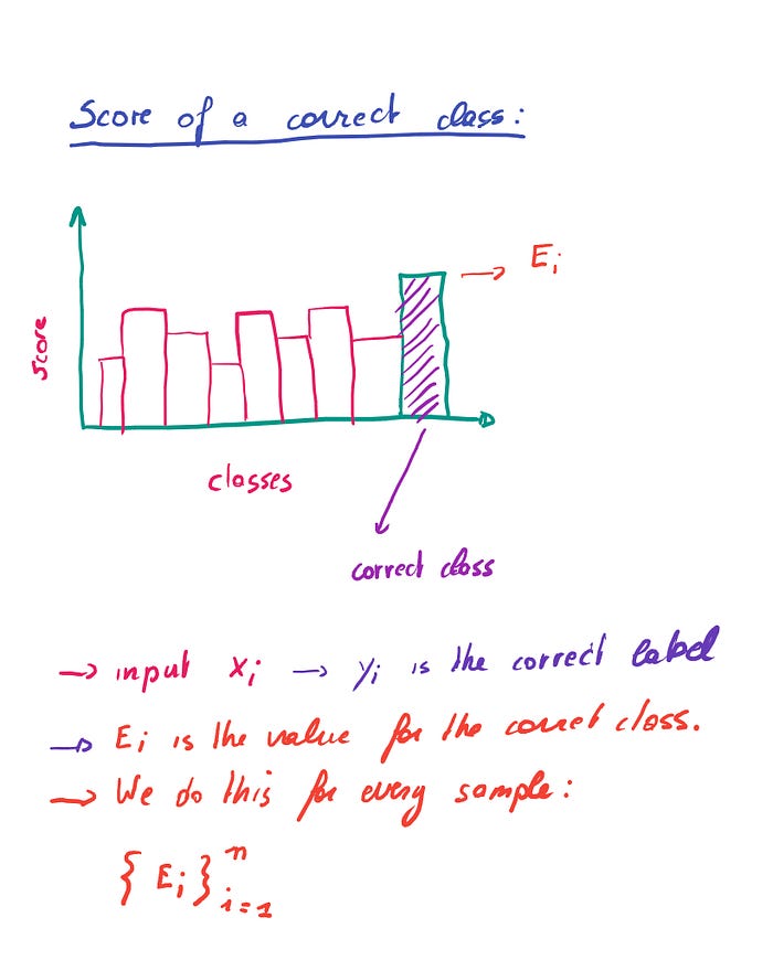
We need to identify the score of a correct class. Let’s say we have a classification problem with 9 classes, then we will get a classification score between 0 and 1 for each of the classes when using a softmax output for a neural network.
Only one of them is correct in our single label classification example below. We call the value for the correct label Eᵢ
When we do this for each sample in the calibration set, then we have a collection of E values of size n (size of our calibration set).

Step 2:
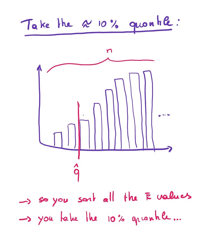
We have a bag of E values of size n and let’s sort them and take the 10% quantile of the n E values. n is not infinite but if it was, then there’s a 90% chance that a new E value would have a value bigger then our 10th quantile.
n is off course finite so we take a small finite sample correction into account for the fact that n is not infinite. This is why we don’t take the exact 10th quantile.

Step 3:
You can take a new prediction where each class has a score and only keep the scores that are above your 10% quantile value and form a set.
Summary :
These 3 steps are the idea behind conformal predictions and this is a very intuitive and powerful concept.
We want our prediction set to have the following qualities:
- The set size should adapt to the difficulty of the prediction (bigger sets for more uncertain predictions)
- The set size should not be too big when not needed
And conformal predictions give use that statistical guarantee and this is true for any algorithm, and dataset, any alpha parameter and any calibration set size if we look at below statement.

(the above should also be 1-alpha on the right side)
The size of your calibration set will have an impact, but you can choose this impact yourself. You can fill in the size of n in de above formule. When our alpha is 0.1 and our n = 100, then we are the chance that our actual value is in the set is between 90% and 91%. If you want to narrow down this interval, then you need to use a bigger calibration set.
This means that using a calibration set of size 100 gives you back enormous statistical guarantees in many situations (distribution free for any dataset / algorithm) and this is impressive.
General framework
We can generalise the above concepts:
- Define a notion of uncertainty (for instance the outcome of your softmax function in a neural network) in your prediction
- Define a score function that uses this notion of uncertainty and gives back a number (in the above example we used the soft max output for the true label).
- Compute q̂ in a way that we correct that we have a finite sample (in the below example we use a calibration set size of 50 and we want 90% confidence (0.1 alpha)

4. Deploy to the prediction set when our score function result for the new datapoint is above q̂
Regression
We discussed a simple classification example, but what about regression problems where you don’t have a notion of uncertainty in the prediction.
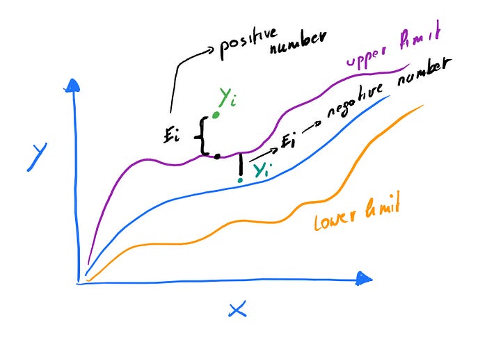
We can use quantile regression to solve this problem where we train 2 models that each have small changes to the loss function and where one model predicts the upper limit and the other predicts the lower limit.

These 2 models estimate quantiles but again we have the same problem. They are an estimate …
But we can use them as our notion of uncertainty.
Step 1:
Our score function is the distance between our boundary line and the actual label. If we have label that is outside the limit, then we have a positive number, if it’s inside the boundary line, then we use a negative number to reflect the distance.

Step 2 and 3:
And now it’s simple. We use the value from the score function and apply the same methodology that we discussed in this article (calculate q̂ and use that to correct the upper/lower limits).
This is a very basic intro in a fascinating field and hopefully you enjoyed this introduction
Sources :
